Meeting Minutes
October 20, 2015
1. Attendees:
- Tom Vercauteren
- Sebastiano Ferraris
- Marc Modat
2. Discussed Topics:
- Numerical methods for the computation of the exponential of an SVF.
(Details below) - Next steps.
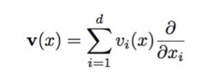
Given an SVF over a domain \Omega (in this case matrix coordinates):
the goal is to find the diffeomorphism \varphi that generated this vector field as its tangent vector field (or velocity field).
This enable to reformulate the problem in terms of solving the differential equations that relates the diffeomorphism and the SVF. Since by definition the field involved is invariant respect to the time, the corresponding differential equation that defines the velocity field is a stationary (or homogeneous) one.
If g is the one parameter subgroup that defines the transformation, the problem of finding g^{1} is equivalent to find the solution to the differential equation:
The operation of integrating the previous differential equation, is in Lie group theory called Lie exponentiation. Therefore
and any numerical method to solve the stationary ODE, become a method to compute the Lie exponential.
The diffeomorphism that defines the solution is computed and represented as a displacement field: the vector field defined at each point of the domain as the difference between the diffeomorphism and the identity computed at this point:
disp(x) = \varphi(x) – x \qquad \forall x \in \Omega
and when the vector field is small enough, the diffeomorphism can be approximated by the SVF itself, when written ad displacement field, so as
\varphi(x) = \exp(v(x)) = v(x) + Id
The poliaffine scaling and squaring is based on this approximation, and on the fact that at point wise the SVF can be approximated by a linear transformation.
Scaling and squaring:
Linear approximation when v is small:
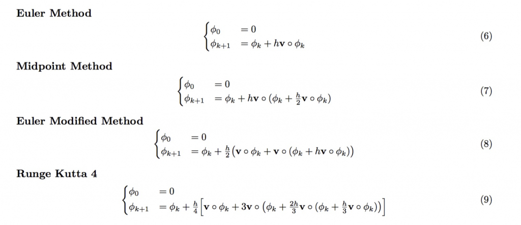
Other methods considered in these experiments are the following:
By a theoretical point of view, these approximation makes sense in the case of diffeomorphism, even if the sum of diffeomorphisms is not defined, because we rely on the displacement field generated by a diffeomorphism.
(Displacement fields are vector fields, whose set is an infinite dimensional space that posses sum, scalar product and norm, otherwise not defined on the group of diffeomorphisms).
Results are considered for an initial set of 200 svn generated by matrices of SE(2), group of rigid body transformations, where the integration can be computed with a closed formula (as the vector field generated by the exponential of the matrix — subtracting the id!).
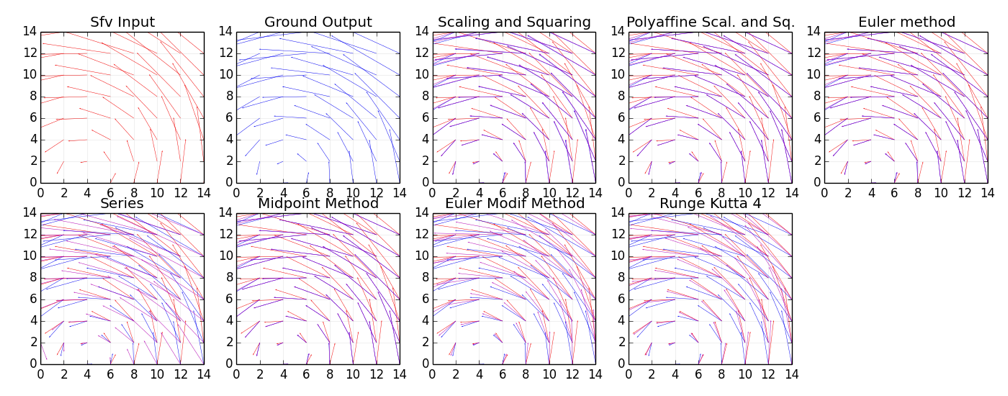
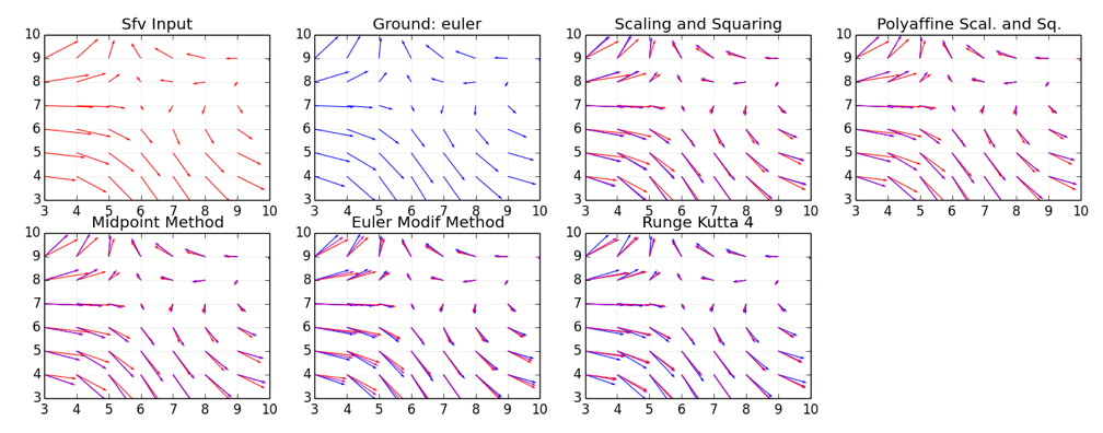
An example of these vector fields are in the following picture
RED: SVF input value.
BLUE: ground truth of the displacement field generated by the diffeomorphisms, our goal.
MAGENTA: solution computed with one of the approximation methods.
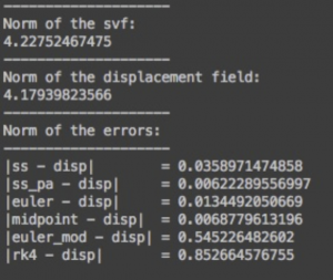
The norm of the error normalised by the square root of the size of the domain are:
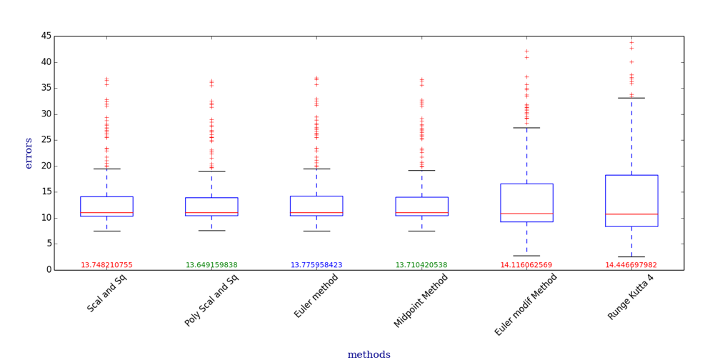
For the dataset of 200 random we have the following box plot, where the error is computed having a ground truth:
(note outliers and y axis values).
In a second set of experiments we used instead a gaussian smoothed random generated SVF, as the one plotted below:
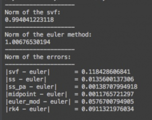
with the following norm of the error for this particular case, where the ground truth has been considered the Euler Method:
(Midpoint method is very similar to the Euler one, this is why so small error).
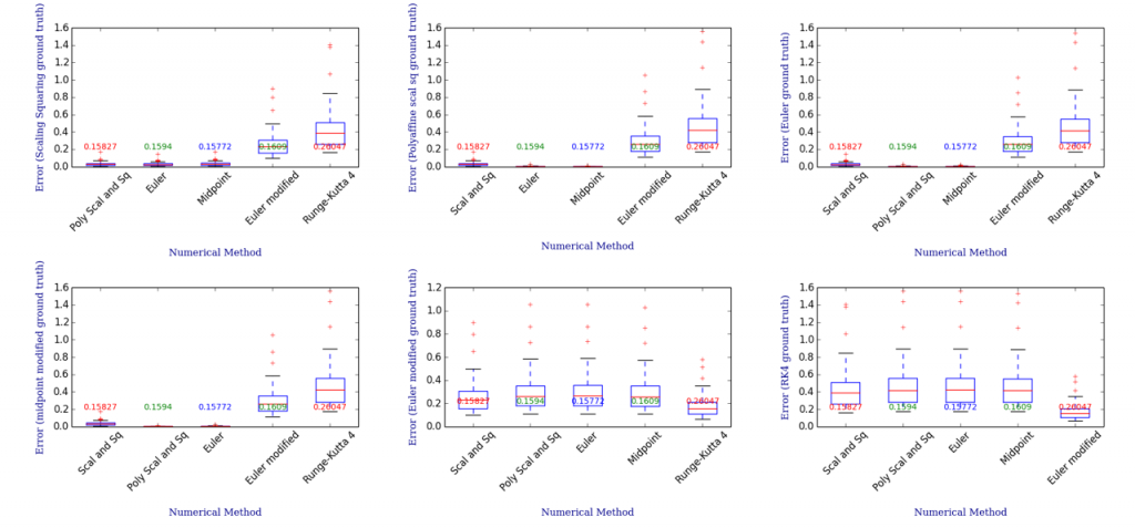
For a dataset of 100 random generated SVF, considering different possible ground truth (not only the Euler method but any method) we have:
Now, the next steps are:
1) correct the value of the norm in the graphic the matrix computation (still debugging!)
2) understand the origin of the outliers, that appears consistently, with almost every time the same ratio over the number of tests (3 every 100).
3) go in deep of each method, theoretically.
4) Add other methods as the Implicit Runge Kutta.
5) Test for different resampling strategies and see what are the improvements that can be made
6) Collect some example of SVF that possesses an analytic integration. Use the analytic diffeomorphisms to have a ground truth in these particular cases.

